Context
In this new post, we’ll be looking at new libraries used to perform clustering (mixture models in particular). In this post you’ll find an introduction to clustering new types of data using MClust.The course is led by Prof.Gilles Durrieu, UBS during the second semester of the uni. year 2021-2022.
About Mclust
In depth documentatin can be foud here : https://mclust-org.github.io/mclust/articles/mclust.html
Extract from the documentation : ‘mclust is a contributed R package for model-based clustering, classification, and density estimation based on finite normal mixture modelling. It provides functions for parameter estimation via the EM algorithm for normal mixture models with a variety of covariance structures, and functions for simulation from these models.’
About Mixture Models
In statistics, a mixture model is a probabilistic model for representing the presence of subpopulations within an overall population, without requiring that an observed data set should identify the sub-population to which an individual observation belongs. Formally a mixture model corresponds to the mixture distribution that represents the probability distribution of observations in the overall population.
Normal Law Mixture
First we’ll take a look at how we can classify normal law samples with mixture models. We’re going to create sample and classes to have decent data.
1
2
# library
library(mclust)
1
2
3
4
## Warning: le package 'mclust' a été compilé avec la version R 4.1.2

## Package 'mclust' version 5.4.9
## Type 'citation("mclust")' for citing this R package in publications.
1
2
3
4
5
6
7
8
9
10
11
12
13
14
15
16
17
18
19
20
21
22
23
# +-----------------------------------------------+
# |                                               |
# |           MIXTURE NORMAL LAW                  |
# |                                               |
# +-----------------------------------------------+

# Normal Law
# Create a sequence of numbers between 0 and 20 incrementing by 1.
# Choose the mean as 1 and standard deviation as 1.

classe1_x <- rnorm(20, 1, 1)
classe1_y <- rnorm(20, 1, 1)

classe2_x <- rnorm(20, 5, 45)
classe2_y <- rnorm(20, 5, 45)

# creating the classes and binding them together to create our dataset
classe1 = cbind(classe1_x, classe1_y, 1)
classe2 = cbind(classe2_x, classe2_y, 2)
data = rbind(classe1, classe2)
# Creating a matrix containing the data 40*2 (40 obs for class 1 and class 2)
sim_matrix = matrix(data, ncol = 3)
head(sim_matrix)
1
2
3
4
5
6
7
##            [,1]      [,2] [,3]
## [1,] -0.4580860 0.8787926    1
## [2,]  2.0038610 1.0968359    1
## [3,]  0.9958816 1.9707677    1
## [4,]  1.2311469 1.2769088    1
## [5,] -0.4513243 1.2053252    1
## [6,]  0.6893095 0.6283313    1
Now that we have our labelled data (which are just 2 classes belonging to 2 different normal laws which you can tweak if you wish) we’re going to cluster the data using HAC.
1
2
3
4
5
6
# HAC
dist_mat = dist(sim_matrix)
fit = hclust(dist_mat, method="ward.D2")

plot(fit, hang=-1, label=sim_matrix[,3])
rect.hclust(fit, k=2, border="red")
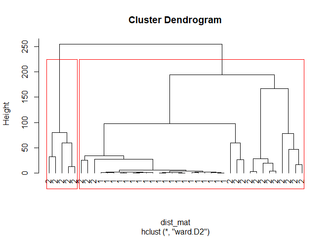 Here we have a clean visualization of our data on a dendrogram. We used k=2 because it’s made up data so we already know the optimal number of clusters. Now let’s use the MClust library :
1
model_mclust = Mclust(sim_matrix[,-3]) #the [,-3] slicing corresponds to all the columns except the last one (which is the label column).
Now that our model is fitted, let’s plot the results :
1
plot(model_mclust, sim_matrix, what="BIC") # fited_model, data, {BIC, clasification, uncertainty etc. }
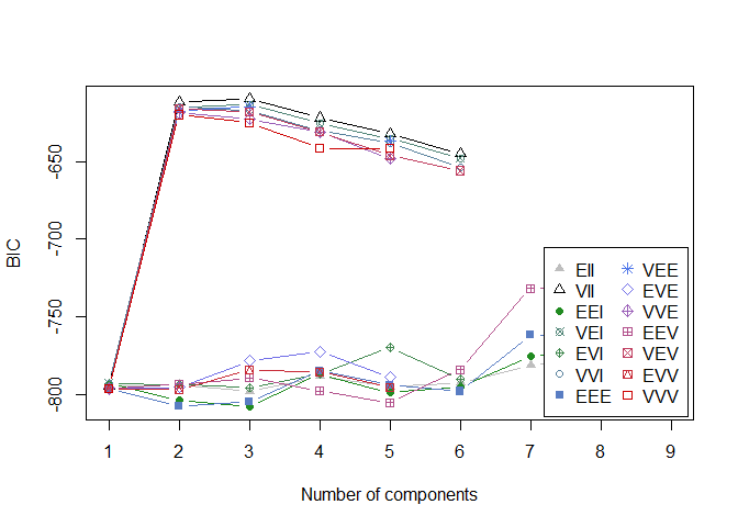
According to the BIC indication, the optimal number of components (clusters) would be 2 (which we already know). The best mixture model is VII : - the model is : Lambda_K (volume) * I (orientation of the clusters). - the volume of each cluster is variable - the distribution of each cluster is on a sphere - the shapes of each cluster are equal
Let’s plot out the classification :
1
2
3
coordProj(sim_matrix[, -3], dimens = c(1,2), what = "classification",
          classification = model_mclust$classification,
          parameters = model_mclust$parameters)
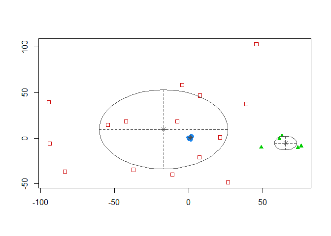 We have 3 clusters with our data being classified in 3 colors. Even if we know that we only have 2 classes. We can assume the error rate isn’t equel to zero. There’s overlapping between the 2 clusters. Let’s check the error rate :
1
2
#error rate
classError(model_mclust$classification, sim_matrix[,3])$errorRate
1
## [1] 0.125
So our classification error rate is 0.125 (it can be 0 sometimes but because the samples are random it changes when you re-run the code). This is because the data is made up and set up to be almost-perfectly classified.
Uniform Law Mixture
Let’s do the same thing as before but we’ll set our data to be 3 classes of random samples of the uniform law :
1
2
3
4
5
6
7
8
9
10
11
12
13
14
15
16
17
18
19
20
21
22
23
24
# +-----------------------------------------------+
# |                                               |
# |           MIXTURE UNIFORM LAW                 |
# |                                               |
# +-----------------------------------------------+

classe1_x <- runif(20, 0, 100)
classe1_y <- runif(20, 0, 100)

classe2_x <- runif(20, 150, 200)
classe2_y <- runif(20, 150, 200)

classe3_x <- runif(20, 250, 260)
classe3_y <- runif(20, 250, 260)

# creating the classes and binding them together to create the dataset
classe1 = cbind(classe1_x, classe1_y, 1)
classe2 = cbind(classe2_x, classe2_y, 2)
classe3 = cbind(classe3_x, classe3_y, 3)
data = rbind(classe1, classe2, classe3)

# Creating a matrix containing the data 40*2 (40 obs for class 1 and class 2)
sim_matrix = matrix(data, ncol = 3)
head(sim_matrix)
1
2
3
4
5
6
7
##           [,1]     [,2] [,3]
## [1,]  5.262265 53.13854    1
## [2,] 62.255513 44.66382    1
## [3,] 25.930816 55.65897    1
## [4,] 80.345403 31.04638    1
## [5,] 31.871906 61.58332    1
## [6,] 13.280975 12.84142    1
Let’s head straight to using Mclust and plot the BIC indicator :
1
2
3
4
#Fitting the model with Mclust for a mixture model
model_mclust = Mclust(sim_matrix[, -3])

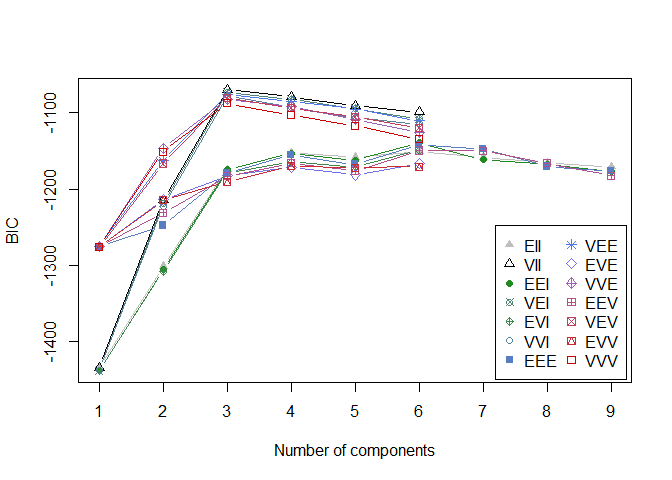
plot(model_mclust, sim_matrix, what = "BIC")
1
2
# we can see that the optimal number of clusters with the BIC criterion is 2 (which is logical since we have 2 classes)
# best mixture model VII for g=2 clusters.
Here we can see that the optimal number of clusters is 3 with the VII model.
Let’s plot the classification and look at the clusters :
1
2
3
coordProj(sim_matrix[, -3], dimens = c(1,2), what = "classification",
          classification = model_mclust$classification,
          parameters = model_mclust$parameters)
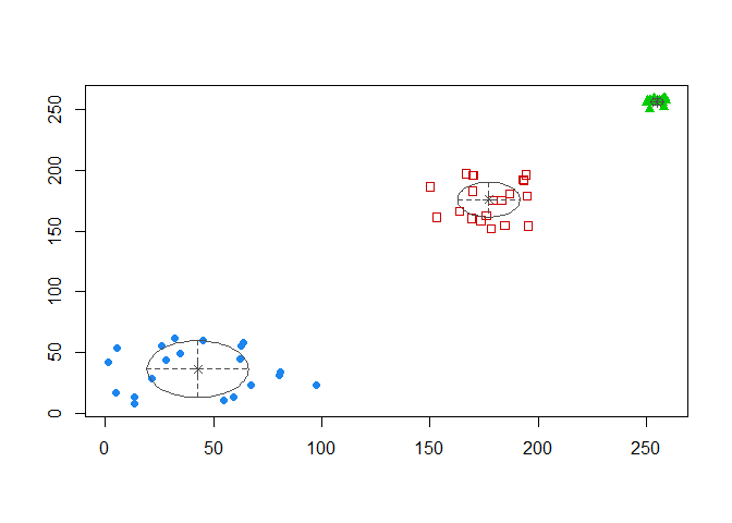 We have our 3 clusters corresponding to our 3 classes with tweaked parameters. This corresponds to the BIC estimation number.
Let’s check our error rate :
1
classError(model_mclust$classification, sim_matrix[,3])$errorRate
1
## [1] 0
Our classification as an error rate slightly superior to 50% which is not great. Bu it’s proof that our data presented high variability and that the method isn’t the best one.
Mixture models applied to real data
We’re going to be using the faithful data (geyser data) and test our mixture models.
1
2
3
4
5
6
7
data('faithful')


#Fitting the model with Mclust for the faithful data model
model_mclust = Mclust(faithful)

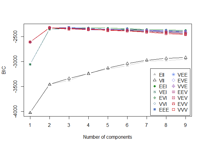
plot(model_mclust, faithful, what = "BIC")
1
2
# we can see that the optimal number of clusters with the BIC criterion is 2 (which is logical since we have 2 classes)
# best mixture model VII for g=2 clusters.
The BIC evaluation plot indicates that the optimal number of components is 2 and the the best fitted model is the EVV model. - the model is : labmda * D_k * A * D_k(transpose) with D_k the orientation of the k-th cluster and A the shape of a cluster. - the volume of each cluster is equal - the distribution of each cluster is on a ellipse - the shapes of each cluster are equal - the orientation of the clusters are variable
1
2
3
coordProj(faithful, dimens = c(1,2), what = "classification",
          classification = model_mclust$classification,
          parameters = model_mclust$parameters)
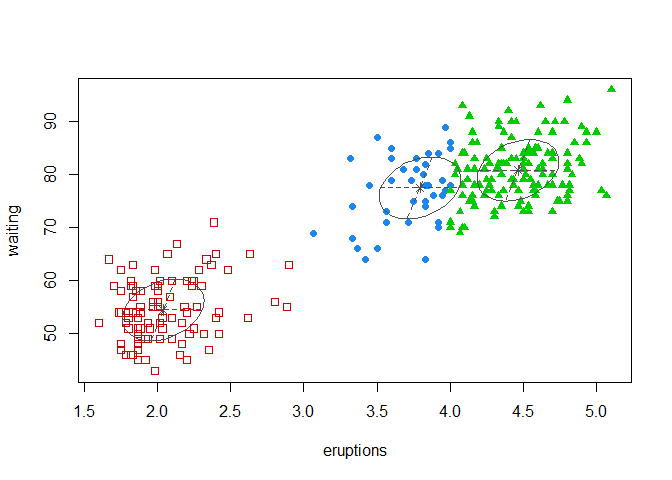
We have 3 clusters, though we have a BIC that indicates that the optimal number of clusters is 2.
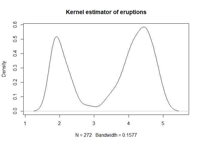
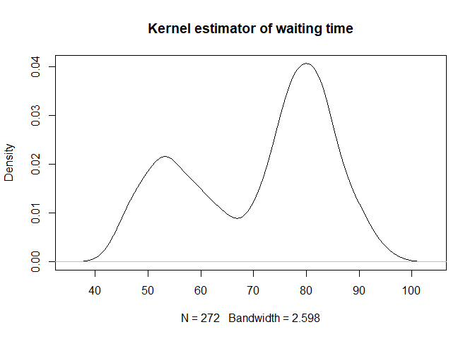
We can plot the density and kernel estimators for each class ;
1
2
3
4
# plotting the density and kernel estimators
# estimaeurs de type de noyau des 2 variables.
library(MASS)
plot(density(faithful[, 1], bw = bw.bcv(faithful[,1])), main="Kernel estimator of eruptions")
1
plot(density(faithful[, 2], bw = bw.bcv(faithful[, 2])), main="Kernel estimator of waiting time")
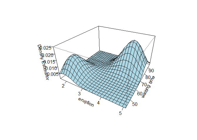
 And finally plot the joint law of the 2 density in perspective :
1
2
3
f1 = kde2d(faithful[, 1], faithful[, 2])
persp(f1, theta=30, phi=30, expand=0.5, col="lightblue",
ticktype="detailed", xlab="eruption", ylab="waiting time", zlab="Density Estimator")
1
contour(f1)
 Even though the classification displayed 3 clusters, we can see that the joint law displays only 2 clusters which corresponds to our BIC estimation using Mclust.
So this concludes our short experience over Mclust which is a very interesting and useful library.
Until next time !
