Bank loan payment default prediction - EOT Assignement
Predicting bank loan payment default in R, from exploratory analysis through to model comparison.
Context
This project is the end of term assignment in the Discriminant Analysis course led by Prof. Salim Lardjane, UBS.
Goals
The project has 2 main goals:
- be familiar with standard machine learning models
- implement from scratch those algorithms to understand the underlying statistics
Loading in the libraries
We’ll be reading a file containing information regarding the financial situation of a person to know weather this person is fit to pay the default or not.
library(foreign)
library(MASS)
library(ROCR)
library(mlogit)
library(caTools)
library(e1071)
library(ggplot2)
library(ROCit)
library("tidyverse")
data <- read.spss("./bankloan.sav",to.data.frame=TRUE)
Descriptive analysis
summary(data)
##       age                                   ed          employ
##  Min.   :20.00   Did not complete high school:460   Min.   : 0.000
##  1st Qu.:29.00   High school degree          :235   1st Qu.: 3.000
##  Median :34.00   Some college                :101   Median : 7.000
##  Mean   :35.03   College degree              : 49   Mean   : 8.566
##  3rd Qu.:41.00   Post-undergraduate degree   :  5   3rd Qu.:13.000
##  Max.   :56.00                                      Max.   :33.000
##     address           income          debtinc         creddebt
##  Min.   : 0.000   Min.   : 13.00   Min.   : 0.10   Min.   : 0.0117
##  1st Qu.: 3.000   1st Qu.: 24.00   1st Qu.: 5.10   1st Qu.: 0.3822
##  Median : 7.000   Median : 35.00   Median : 8.70   Median : 0.8851
##  Mean   : 8.372   Mean   : 46.68   Mean   :10.17   Mean   : 1.5768
##  3rd Qu.:12.000   3rd Qu.: 55.75   3rd Qu.:13.80   3rd Qu.: 1.8984
##  Max.   :34.000   Max.   :446.00   Max.   :41.30   Max.   :20.5613
##     othdebt         default       preddef1            preddef2
##  Min.   : 0.04558   No  :517   Min.   :0.0001166   Min.   :0.0000387
##  1st Qu.: 1.04594   Yes :183   1st Qu.:0.0456301   1st Qu.:0.0351757
##  Median : 2.00324   NA's:150   Median :0.1715129   Median :0.1590730
##  Mean   : 3.07879              Mean   :0.2585762   Mean   :0.2578660
##  3rd Qu.: 3.90300              3rd Qu.:0.4073259   3rd Qu.:0.4332770
##  Max.   :35.19750              Max.   :0.9993967   Max.   :0.9994570
##     preddef3
##  Min.   :0.07464
##  1st Qu.:0.13476
##  Median :0.20010
##  Mean   :0.25858
##  3rd Qu.:0.32863
##  Max.   :0.94810
Discriminant Analysis without cross-validation
Separating the data (train/test)
library(MASS)
library(e1071)

na <- c(701:850)
apred <- data[na,] # the data that we're going to predict later on, once our models are trained
data2 <- subset(data, data$default != "NA'S") # the data we'll use for the train/test datasets
data2<-data2[1:9]
data2<-data2[-2]
data2[,8]<-as.numeric(data2$default)-1
n = dim(data2)[1]

id = sample(1:n,floor(0.75*n),replace=F)
train <- data2[id,]
test <- data2[-id,]
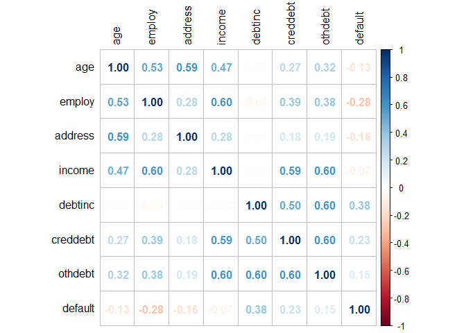
Correlation coefficient visualization
library(corrplot)
corrplot(cor(train),        # Correlation matrix
         method = "number", # Correlation plot method
         type = "full",    # Correlation plot style (also "upper" and "lower")
         diag = TRUE,      # If TRUE (default), adds the diagonal
         tl.col = "black", # Labels color
         bg = "white",     # Background color
         title = "",       # Main title
         col = NULL)       # Color palette
Graphs
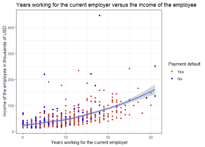
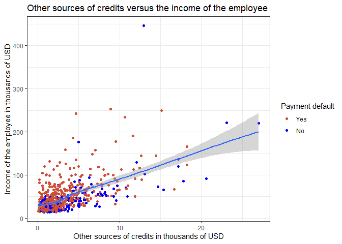
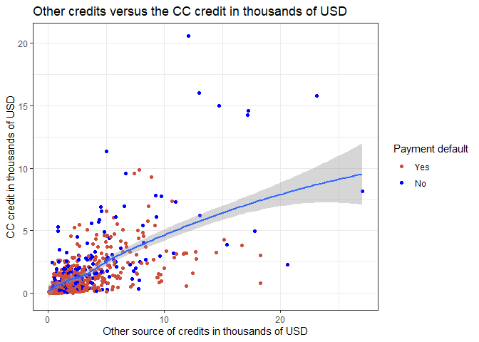
In order to find the best way to represent our data, we’ll sort the variables in 3 classes : stability, demographic and financial data.
# stability variables : employ address
# demographic variables : age
# financial variables : income debtinc creddebt othdebt

# employ income

data2 %>% mutate(default = factor(default)) %>%
  ggplot(aes(x = employ, y = income)) +
  geom_point(mapping = aes(color = default)) +
  labs(x=" Years working for the current employer",
       y=" Income of the employee in thousands of USD",
       color = "Payment default") +
  geom_smooth() +
  scale_color_manual(values = c("0" = "tomato3",
                                "1" = "blue"),
                     labels = c("Yes",
                               "No")) +
  theme_bw()+
  ggtitle("Years working for the current employer versus the income of the employee")
# othdebt income

data2 %>% mutate(default = factor(default)) %>%
  ggplot(aes(x = othdebt, y = income)) +
  geom_point(mapping = aes(color = default)) +
  labs(y="Income of the employee in thousands of USD",
       x="Other sources of credits in thousands of USD",
       color = "Payment default") +
  geom_smooth() +
  scale_color_manual(values = c("0" = "tomato3",
                                "1" = "blue"),
                     labels = c("Yes",
                               "No")) +
  theme_bw()+
  ggtitle("Other sources of credits versus the income of the employee")
# othdebt creddebt

data2 %>% mutate(default = factor(default)) %>%
  ggplot(aes(x = othdebt, y = creddebt)) +
  geom_point(mapping = aes(color = default)) +
  labs(y="CC credit in thousands of USD",
       x="Other source of credits in thousands of USD",
       color = "Payment default") +
  geom_smooth() +
  scale_color_manual(values = c("0" = "tomato3",
                                "1" = "blue"),
                     labels = c("Yes",
                               "No")) +
  theme_bw()+
  ggtitle("Other credits versus the CC credit in thousands of USD")
Defining the ROC function
This function will allow us to trace a ROC curve for each model that returns posterior probabilities
roc <- function(post1, col){
  trapeze <- function(ao,bo) {
    k <- length(ao)
    iz <- 0
    for (i in 1:(k-1)) {
      iz <- iz+(ao[i+1]-ao[i])*(bo[i]+bo[i+1])/2
    }
    return(iz)
  }
  delta=0.001
  valeurs <- seq(0,1,delta)
  N <- length(valeurs)
  sensibilite <- rep(NA,N)
  antispec <- rep(NA,N)
  i <- 0
  for (u in valeurs) {
    i <- i+1
    pr2predict <- (post1>u)+0

    TN1 <- sum((pr2predict==0)*(test$default==0))
    FP1 <- sum((pr2predict==1)*(test$default==0))
    FN1 <- sum((pr2predict==0)*(test$default==1))
    TP1 <- sum((pr2predict==1)*(test$default==1))

    Rap1 <- TP1/(TP1+FN1)
    Pre1 <- TP1/(TP1+FP1)
    F_sco1 <- (2*TP1)/(2*TP1+FP1+FN1)
    Spe1 <- TN1/(FP1+TN1)
    Err1 <- ((FP1+FN1)/(TN1+FP1+TP1+FN1)*100)

    sensibilite[i] <- Rap1
    antispec[i] <- 1-Spe1
  }
  antispec<- c(0,rev(antispec),1)
  sensibilite <- c(0,rev(sensibilite),1)
  plot(antispec,sensibilite,type="s",col=col,lwd=1)

  return(trapeze(antispec, sensibilite))
}
Defining the models
For each model we’ll compute recall, f-score, acc, specificity and add the values to a dataframe that we’ll comment at the end.
Closest Mean method
no.age <- mean(train[train$default==0,]$age)
yes.age <- mean(train[train$default==1,]$age)
no.employ <- mean(train[train$default==0,]$employ)
yes.employ <- mean(train[train$default==1,]$employ)
no.address <- mean(train[train$default==0,]$address)
yes.address <- mean(train[train$default==1,]$address)
no.income <- mean(train[train$default==0,]$income)
yes.income <- mean(train[train$default==1,]$income)
no.debtinc <- mean(train[train$default==0,]$debtinc)
yes.debtinc <- mean(train[train$default==1,]$debtinc)
no.creddebt <- mean(train[train$default==0,]$creddebt)
yes.creddebt <- mean(train[train$default==1,]$creddebt)
no.othdebt <- mean(train[train$default==0,]$othdebt)
yes.othdebt <- mean(train[train$default==1,]$othdebt)

prediction <- function(x,y,z,a,b,c,d) {
 if ((x-yes.age)^2+(y-yes.employ)^2+(z-yes.address)^2+(a-yes.income)^2+(b-yes.debtinc)^2+(c-yes.creddebt)^2+(d-yes.othdebt)^2 >(x-no.age)^2+(y-no.employ)^2+(z-no.address)^2+(a-no.income)^2+(b-no.debtinc)^2+(c-no.creddebt)^2+(d-no.othdebt)^2)
 {
 return(1)
 } else {return(0)}
}

pred <- rep(NA,length(test$default))
for (i in 1:length(test$default)) {
 pred[i] <- prediction(test$age[i],test$employ[i],test$address[i], test$income[i], test$debtinc[i], test$creddebt[i], test$othdebt[i])
}

MCPPM = table(pred,test$default)
MCPPMerr = (MCPPM[2,1]+MCPPM[1,2])/sum(MCPPM)
MCPPMrappel = MCPPM[2,2]/(MCPPM[2,2]+MCPPM[1,2])
MCPPMprecision = MCPPM[2,2]/(MCPPM[2,2]+MCPPM[2,1])
MCPPMF = 2*MCPPM[2,2]/(2*MCPPM[2,2]+MCPPM[2,1]+2*MCPPM[1,2])
MCPPMspecificite = MCPPM[2,2]/(MCPPM[2,2]+MCPPM[2,1])

PPM = round(c(MCPPMerr,MCPPMrappel,MCPPMprecision,MCPPMF,MCPPMspecificite),2)
Quadratic Discriminant Analysis method
library(MASS)
model = predict(qda(default~.,train),test)

MCqda = table(test$default,model$class) # correlation matrix

MCqdaerr = (MCqda[2,1]+MCqda[1,2])/sum(MCqda)
MCqdarappel = MCqda[2,2]/(MCqda[2,2]+MCqda[1,2])
MCqdaprecision = MCqda[2,2]/(MCqda[2,2]+MCqda[2,1])
MCqdaF = 2*MCqda[2,2]/(2*MCqda[2,2]+MCqda[2,1]+2*MCqda[1,2])
MCqdaspecificite = MCqda[2,2]/(MCqda[2,2]+MCqda[2,1])
qda = round(c(MCqdaerr,MCqdarappel,MCqdaprecision,MCqdaF,MCqdaspecificite),2)
Linear Discriminant Analysis method
library(MASS)
model = predict(lda(default~.,train),test)

MClda = table(test$default,model$class)

MCldaerr = (MClda[2,1]+MClda[1,2])/sum(MClda)
MCldarappel = MClda[2,2]/(MClda[2,2]+MClda[1,2])
MCldaprecision = MClda[2,2]/(MClda[2,2]+MClda[2,1])
MCldaF = 2*MClda[2,2]/(2*MClda[2,2]+MClda[2,1]+2*MClda[1,2])
MCldaspecificite = MClda[2,2]/(MClda[2,2]+MClda[2,1])
lda = round(c(MCldaerr,MCldarappel,MCldaprecision,MCldaF,MCldaspecificite),2)
Naive Bayes method
library(e1071)
model = predict(naiveBayes(default~.,train),test)

MCbayes = table(test$default,model)

MCbayeserr = (MCbayes[2,1]+MCbayes[1,2])/sum(MCbayes)
MCbayesrappel = MCbayes[2,2]/(MCbayes[2,2]+MCbayes[1,2])
MCbayesprecision = MCbayes[2,2]/(MCbayes[2,2]+MCbayes[2,1])
MCbayesF = 2*MCbayes[2,2]/(2*MCbayes[2,2]+MCbayes[2,1]+2*MCbayes[1,2])
MCbayesspecificite = MCbayes[2,2]/(MCbayes[2,2]+MCbayes[2,1])
bayes = round(c(MCbayeserr,MCbayesrappel,MCbayesprecision,MCbayesF,MCbayesspecificite),2)
K closest neighbours method
library(class)
cl <- as.factor(train$default)

predtest <- knn(train,test,cl, k=1)

MCknn1 = table(test$default,predtest)

MCknn1err = (MCknn1[2,1]+MCknn1[1,2])/sum(MCknn1)
MCknn1rappel = MCknn1[2,2]/(MCknn1[2,2]+MCknn1[1,2])
MCknn1precision = MCknn1[2,2]/(MCknn1[2,2]+MCknn1[2,1])
MCknn1F = 2*MCknn1[2,2]/(2*MCknn1[2,2]+MCknn1[2,1]+2*MCknn1[1,2])
MCknn1specificite = MCknn1[2,2]/(MCknn1[2,2]+MCknn1[2,1])

knn1 = round(c(MCknn1err,MCknn1rappel,MCknn1precision,MCknn1F,MCknn1specificite),2)


predtest <- knn(train,test,cl, k=2)

MCknn2 = table(test$default,predtest)

MCknn2err = (MCknn2[2,1]+MCknn2[1,2])/sum(MCknn2)
MCknn2rappel = MCknn2[2,2]/(MCknn2[2,2]+MCknn2[1,2])
MCknn2precision = MCknn2[2,2]/(MCknn2[2,2]+MCknn2[2,1])
MCknn2F = 2*MCknn2[2,2]/(2*MCknn2[2,2]+MCknn2[2,1]+2*MCknn2[1,2])
MCknn2specificite = MCknn2[2,2]/(MCknn2[2,2]+MCknn2[2,1])

knn2 = round(c(MCknn2err,MCknn2rappel,MCknn2precision,MCknn2F,MCknn2specificite),2)

predtest <- knn(train,test,cl,k=3)

MCknn3 = table(test$default,predtest)

MCknn3err = (MCknn3[2,1]+MCknn3[1,2])/sum(MCknn3)
MCknn3rappel = MCknn3[2,2]/(MCknn3[2,2]+MCknn3[1,2])
MCknn3precision = MCknn3[2,2]/(MCknn3[2,2]+MCknn3[2,1])
MCknn3F = 2*MCknn3[2,2]/(2*MCknn3[2,2]+MCknn3[2,1]+2*MCknn3[1,2])
MCknn3specificite = MCknn3[2,2]/(MCknn3[2,2]+MCknn3[2,1])

knn3 = round(c(MCknn3err,MCknn3rappel,MCknn3precision,MCknn3F,MCknn3specificite),2)
Logistic regression model
Preparing the data
data2$default <- as.factor(data2$default)
Defining the model
reglog <- glm(default~., family = binomial, data=train, control=list(maxit=1000, trace=TRUE, epsilon=1e-16))

preds <- predict(reglog, test, type='response')
optimal_cutoff <- ifelse(preds > 0.5, 1, 0)

summary(reglog)
##
## Call:
## glm(formula = default ~ ., family = binomial, data = train, control = list(maxit = 1000,
##     trace = TRUE, epsilon = 1e-16))
##
## Deviance Residuals:
##     Min       1Q   Median       3Q      Max
## -2.3241  -0.6734  -0.3020   0.2628   2.6057
##
## Coefficients:
##              Estimate Std. Error z value Pr(>|z|)
## (Intercept) -1.657904   0.664307  -2.496   0.0126 *
## age          0.044607   0.020375   2.189   0.0286 *
## employ      -0.268156   0.037089  -7.230 4.82e-13 ***
## address     -0.113424   0.027131  -4.181 2.91e-05 ***
## income      -0.008652   0.008473  -1.021   0.3072
## debtinc      0.067861   0.035900   1.890   0.0587 .
## creddebt     0.611694   0.134228   4.557 5.19e-06 ***
## othdebt      0.080870   0.085357   0.947   0.3434
## ---
## Signif. codes:  0 '***' 0.001 '**' 0.01 '*' 0.05 '.' 0.1 ' ' 1
##
## (Dispersion parameter for binomial family taken to be 1)
##
##     Null deviance: 602.75  on 524  degrees of freedom
## Residual deviance: 418.16  on 517  degrees of freedom
## AIC: 434.16
##
## Number of Fisher Scoring iterations: 7
#confusion matrix
MCreg = table(test$default, optimal_cutoff)

MCregerr = (MCreg[2,1]+MCreg[1,2])/sum(MCreg)
MCregrappel = MCreg[2,2]/(MCreg[2,2]+MCreg[1,2])
MCregprecision = MCreg[2,2]/(MCreg[2,2]+MCreg[2,1])
MCregF = 2*MCreg[2,2]/(2*MCreg[2,2]+MCreg[2,1]+2*MCreg[1,2])
MCregspecificite = MCreg[2,2]/(MCreg[2,2]+MCreg[2,1])
reg = round(c(MCregerr,MCregrappel,MCregprecision,MCregF,MCregspecificite),2)
titles = c("Error rate","Recall","Accuracy","F-Score","Specificity")
data.frame(titles,lda,qda,knn1,knn2,knn3,PPM, reg)
##        titles  lda  qda knn1 knn2 knn3  PPM  reg
## 1  Error rate 0.19 0.21 0.29 0.30 0.24 0.54 0.18
## 2      Recall 0.70 0.66 0.46 0.42 0.56 0.22 0.68
## 3    Accuracy 0.50 0.46 0.46 0.35 0.39 0.14 0.59
## 4     F-Score 0.52 0.47 0.36 0.30 0.39 0.13 0.55
## 5 Specificity 0.50 0.46 0.46 0.35 0.39 0.14 0.59
Disciminant Analysis with cross-validation method Leave-One-Out
data2$default <- as.numeric(data2$default)-1

n = dim(data2)[1]
lda = 0
qda = 0
naive = 0
knn1 = 0
knn2 = 0
knn3 = 0
ppm = 0

for(i in 1:n) {


  train <- data2[-i,]
  test <- data2[i,]

  # LDA #

  model = predict(lda(default~.,train),test)
  erlda = (data2$default[i] != model$class) + 0
  MClda = table(model$class,test$default)

  lda[i] = erlda

  # QDA #

  model2 = predict(qda(default~.,train),test)
  erqda = (data2$default[i] != model2$class) + 0

  qda[i] = erqda

  # Naive Bayes #

  model3 = predict(naiveBayes(default~.,train),test)
  ernaive = (data2$default[i] != model3) + 0

  naive[i] = ernaive

  # KNN #

  cl <- as.factor(train$default)

  # Prediction K=1 #
  predtest <- knn(train,test,cl, k=1)

  # errors K=1 #
  erknn1 = (data2$default[i] != predtest) + 0
  knn1[i] = erknn1

  # Prediction K=2 #
  predtest <- knn(train,test,cl, k=2)

  # errors K=2 #
  erknn2 = (data2$default[i] != predtest) + 0
  knn2[i] = erknn2

  # Prediction K=3 #
  predtest <- knn(train,test,cl, k=3)

  # errors K=3 #
  erknn3 = (data2$default[i] != predtest) + 0
  knn3[i] = erknn3

  # Prediction for closest mean #

  no.age <- mean(train[train$default==0,]$age)
  yes.age <- mean(train[train$default==1,]$age)
  no.employ <- mean(train[train$default==0,]$employ)
  yes.employ <- mean(train[train$default==1,]$employ)
  no.address <- mean(train[train$default==0,]$address)
  yes.address <- mean(train[train$default==1,]$address)
  no.income <- mean(train[train$default==0,]$income)
  yes.income <- mean(train[train$default==1,]$income)
  no.debtinc <- mean(train[train$default==0,]$debtinc)
  yes.debtinc <- mean(train[train$default==1,]$debtinc)
  no.creddebt <- mean(train[train$default==0,]$creddebt)
  yes.creddebt <- mean(train[train$default==1,]$creddebt)
  no.othdebt <- mean(train[train$default==0,]$othdebt)
  yes.othdebt <- mean(train[train$default==1,]$othdebt)

  prediction <- function(x,z,a,b,c,d,e) {
   if ((x-yes.age)^2+(z-yes.employ)^2+(a-yes.address)^2+
       (b-yes.income)^2+(c-yes.debtinc)^2+(d-yes.creddebt)^2+
       (e-yes.othdebt)^2 >
       (x-no.age)^2+(z-no.employ)^2+(a-no.address)^2+
       (b-no.income)^2+(c-no.debtinc)^2+(d-no.creddebt)^2+
       (e-no.othdebt)^2)
  {
   return(1)
   } else {return(0)}
  }

  pred <- prediction(test$age,test$employ,test$address, test$income, test$debtinc, test$creddebt, test$othdebt)

  erppm = (data2$default[i] != pred) + 0
  ppm[i] <- erppm
}

validationCroisée = c("taux d'erreur")
res = c(mean(lda),mean(qda),mean(naive),mean(knn1),mean(knn2),mean(knn3), mean(ppm))
lda = mean(lda)
qda = mean(qda)
naive = mean(naive)
knn1 = mean(knn1)
knn2 = mean(knn2)
knn3 = mean(knn3)
ppm = mean(ppm)
data.frame(validationCroisée,lda,qda,naive,knn1,knn2,knn3,ppm)
##   validationCroisée       lda       qda     naive      knn1      knn2      knn3
## 1     taux d'erreur 0.1871429 0.2228571 0.2471429 0.2842857 0.2928571 0.2471429
##         ppm
## 1 0.5414286
Here we can see that the model with the smallest error rate is the LDA model.
Using our best model for the prediction on the data
model = predict(lda(default~.,data2),apred)
model$class
##   [1] 0 0 1 0 0 0 0 1 0 0 0 0 0 0 0 1 1 0 1 0 0 0 0 0 0 0 0 0 0 0 0 0 1 0 0 0 0
##  [38] 0 0 0 0 0 0 0 0 1 0 0 0 0 0 0 0 0 0 0 0 0 0 0 0 0 0 1 0 0 0 0 0 0 1 0 0 1
##  [75] 0 0 0 0 0 0 0 1 0 1 1 0 0 0 0 1 0 0 0 0 0 0 0 0 0 1 0 1 0 1 0 0 0 1 0 0 1
## [112] 0 0 0 0 0 0 0 0 0 0 0 1 0 0 0 1 0 0 0 0 0 0 0 0 0 1 0 0 0 1 0 0 0 0 0 0 0
## [149] 0 0
## Levels: 0 1
yes = 0
no = 0
for (i in 1:150){
  if(model$class[i] == 1){
    yes=yes+1
  }else{
    no=no+1
  }
}
yes
## [1] 23
no
## [1] 127
prediction = yes/150;prediction
## [1] 0.1533333
So out of 150 people, 23 are likely to repay their credit and 127 are not likely to repay their credit, iow -> 15.3% of the population